Wasserstein Embedding for Graph Learning
1: HRL Laboratories, LLC 2: University of Virginia
∗ denotes equal contribution
Abstract
We present Wasserstein Embedding for Graph Learning (WEGL), a novel and fast framework for embedding entire graphs in a vector space, in which various machine learning models are applicable for graph-level prediction tasks. We leverage new insights on defining similarity between graphs as a function of the similarity between their node embedding distributions. Specifically, we use the Wasserstein distance to measure the dissimilarity between node embeddings of different graphs. Different from prior work, we avoid pairwise calculation of distances between graphs and reduce the computational complexity from quadratic to linear in the number of graphs. WEGL calculates Monge maps from a reference distribution to each node embedding and, based on these maps, creates a fixed-sized vector representation of the graph. We evaluate our new graph embedding approach on various benchmark graph-property prediction tasks, showing state-of-the-art classification performance, while having superior computational efficiency.
Contributions
Method Description
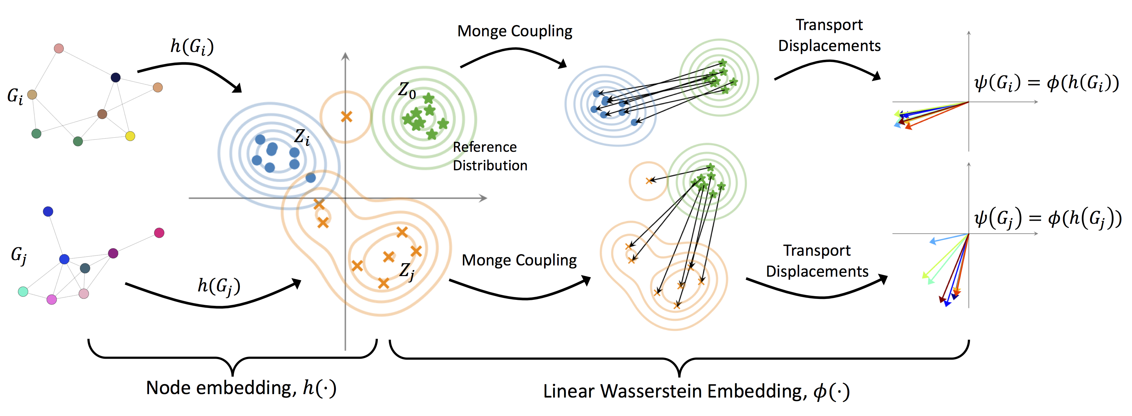
WEGL consists of two stages: 1) node embedding of a graph, 2) linear Wasserstein embedding of the embedded nodes. Below, we describe each of these embeddings.
Node Embedding
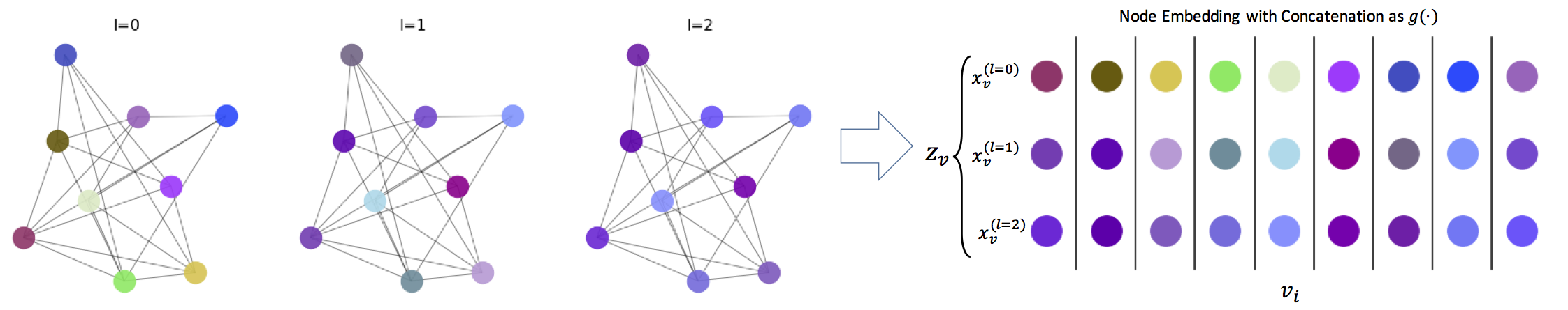
There are many choices for node embedding methods [2]. These methods in general could be parametric or non-parametric, for instance, as in propagation/diffusion-based embeddings. Parametric embeddings are often implemented via a GNN encoder. The encoder can capture different graph properties depending on the type of supervision (e.g., supervised or unsupervised). Among the recent work on this topic, self-supervised embedding methods have been shown to be promising [3].
For our node embedding process, $h(\cdot)$, we follow a similar non-parametric propagation/diffusion-based encoder as in [1]. One of the appealing advantages of this framework is its simplicity, as there are no trainable parameters involved. In short, given a graph $G=(\mathcal{V},\mathcal{E})$ with node features $\{x_v\}_{v\in\mathcal{V}}$ and scalar edge features $\{w_{uv}\}_{(u,v)\in\mathcal{E}}$, we use:
Linear Wasserstein Embedding
Linear Wasserstein embedding [5,6] provides an explicit isometric Hilbertian embedding of probability distributions such that the Euclidean distance between the embedded distributions approximates the 2-Wasserstein distance, $\mathcal{W}_2$. We adhere to the definition of the linear Wasserstein embedding for continuous measures. However, all derivations hold for discrete measures as well. More precisely, let $\mu_0$ be a reference probability measure defined on $\mathcal{Z}\subseteq \mathbb{R}^d$, with a positive probability density function $p_0$, s.t. $d\mu_0(z)=p_0(z)dz$ and $p_0(z)>0$ for $\forall z \in \mathcal{Z}$. Let $f_i$ denote the Monge map that pushes $\mu_0$ into $\mu_i$, i.e., \begin{align} f_i=\operatorname{argmin}_{f\in MP(\mu_0,\mu_i)} \int_\mathcal{Z}\|z-f(z)\|^2d\mu_0(z). \end{align}
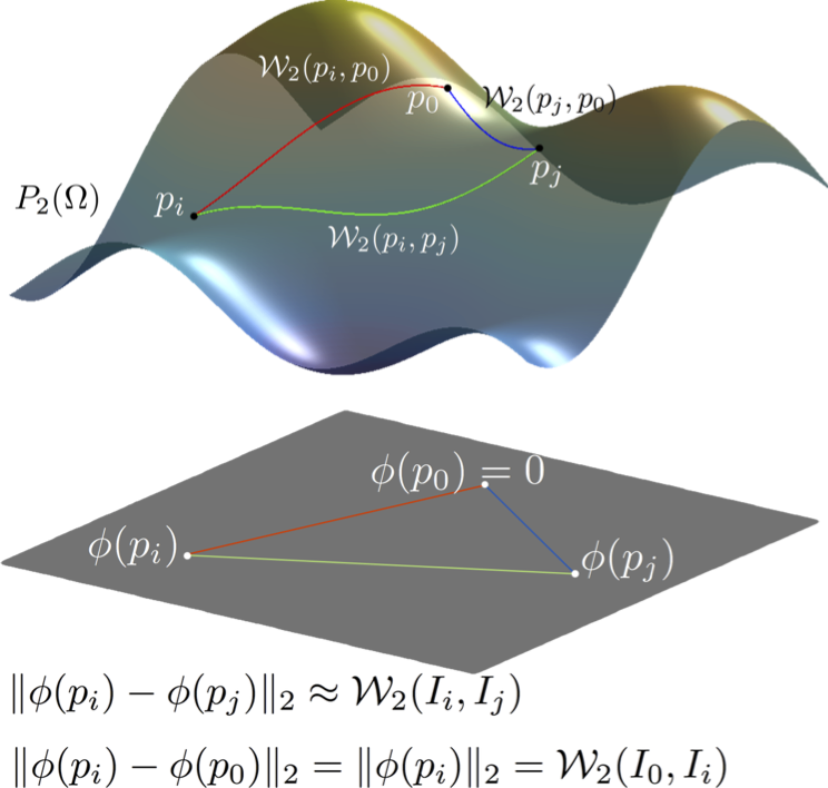
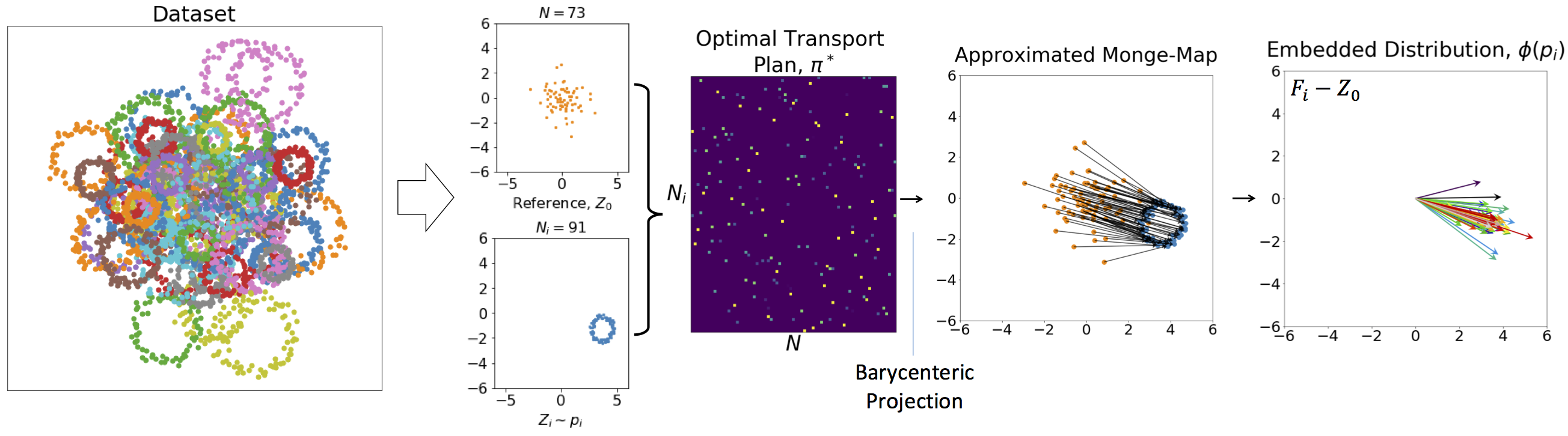
Discrete Measures: Consider a set of probability distributions $\{p_i\}_{i=1}^M$, and let $Z_i = \big[ z^i_1, \dots , z^i_{N_i} \big]^T \in \mathbb{R}^{N_i\times d}$ be an array containing $N_i$ i.i.d. samples from distribution $p_i$, i.e., $z^i_k \in \mathbb{R}^d \sim p_i, \forall k\in\{1, \dots, N_i\}$. Let us define $p_0$ to be a reference distribution, with $Z_0 = \big[ z^0_1, \dots , z^0_{N} \big]^T \in \mathbb{R}^{N \times d}$ , where $N=\lfloor \frac{1}{M}\sum_{i=1}^M N_i \rfloor$ and $z^0_j \in \mathbb{R}^d \sim p_0, \forall j\in\{1, \dots, N\}$. The optimal transport plan between $p_i$ and $p_0$, denoted by $\pi_i^*\in \mathbb{R}^{N\times N_i}$, is the solution to the following linear program, \vspace{-.05in} \begin{equation} \pi_i^* = \operatorname{argmin}_{\pi\in \Pi_i}~\sum_{j=1}^{N}\sum_{k=1}^{N_i} \pi_{jk}\| z^0_j - z^i_k \|^2, \end{equation} where $\Pi_i\triangleq\Big\{\pi \in \mathbb{R}^{N\times N_i}~\big|~N_i\sum\limits_{j=1}^N \pi_{jk}=N\sum\limits_{k=1}^{N_i} \pi_{jk}=1,~\forall k\in\{1, \dots, N_i\}, \forall j\in\{1, \dots, N\}\Big\}$. The Monge map is then approximated from the optimal transport plan by barycentric projection via \begin{align} F_i= N(\pi_i^* Z_i)\in \mathbb{R}^{N\times d}. \end{align} Finally, the embedding can be calculated by $\phi(Z_i)=(F_i-Z_0)/\sqrt{N}\in \mathbb{R}^{N\times d}$. With a slight abuse of notation, we use $\phi(p_i)$ and $\phi(Z_i)$ interchangeably throughout the paper. Due to the barycenteric projection, here, $\phi(\cdot)$ is only pseudo-invertible.
Numerical Demonstration: Consider $Z_i = \big[ z^i_1, \dots , z^i_{N_i} \big]^T \in \mathbb{R}^{N_i\times d}$ be samples from scaled and translated ring distributions (as shown below), and let us set the reference distribution to a normal distribution. The figure below shows the optimal transport plan, the result of the barycentric projection to approximate the Monge plan, and the final embedding.
To demonstrate the modeling capability of the framework, we calculate the mean in the embedding space (i.e., on the vector fields), and invert it to obtain the mean distribution $\bar{p}$. The figure below shows the calculated mean, indicating that the linear Wasserstein embedding framework has successfully retrieved a ring distribution as the mean. Finally, we calculate Euclidean geodesics in the embedding space (i.e., the convex combination of the vector fields) between $p_i$ and $p_0$, as well as between $p_i$ and $p_j$, and show the inverted geodesics below.
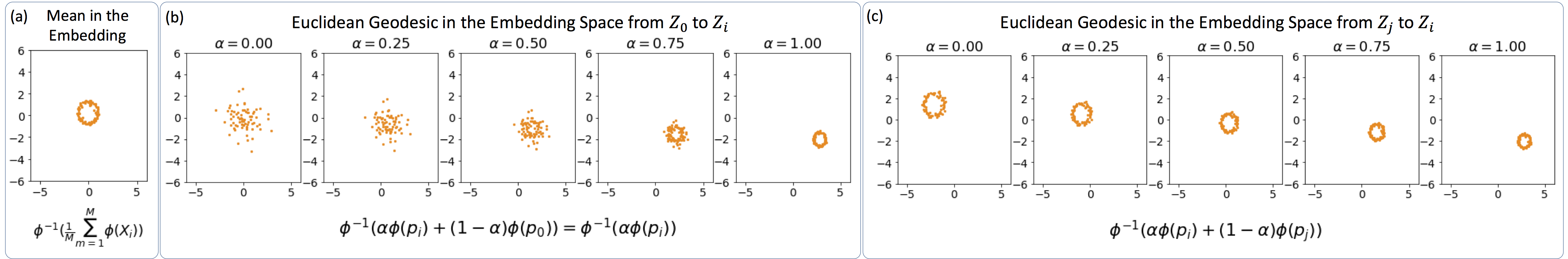
As the figures demosntrate, the calculated geodesics follow the Wasserstein geodesics, and the linear Wasserstein embedding provides a nonlinear modeling of the distributions. The code to regenerate these demonstration can be found here.
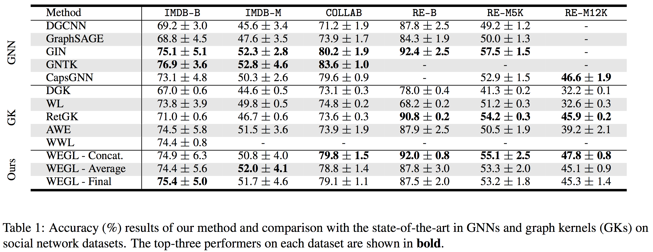
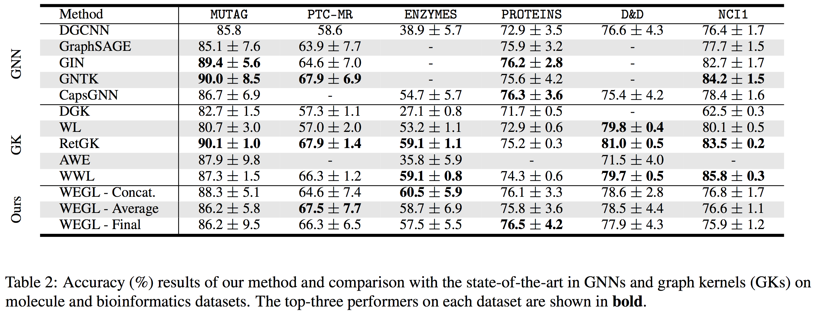
Results
Here we compare the performance of WEGL on TUD benchmark datasets with the state-of-the-art in GNNs and graph kernels (GKs).
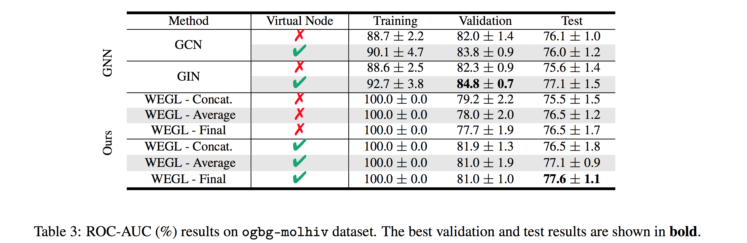
We also tested our algorithm on the molecular property prediction task on the ogbg-molhiv dataset [7]. Table 3 (below) shows the performance of WEGL on this dataset (Link to Leaderboard).
Computation Time
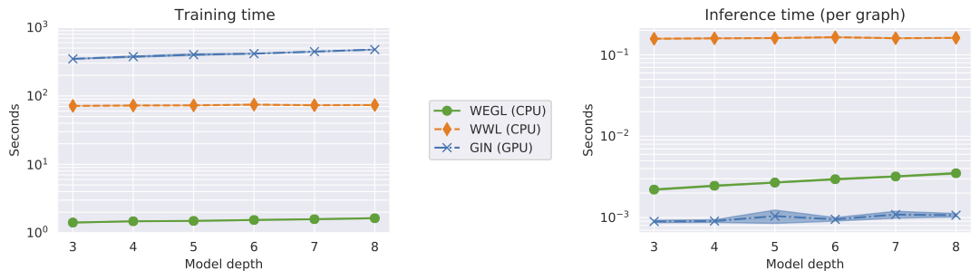
We compared the algorithmic efficiency of WEGL with GIN and the Wasserstein Weisfeiler-Lehman (WWL) graph kernel. For this experiment, we used the IMDB-BINARY dataset and measured the wall-clock training and inference times for the three methods (to achieve results reported in Table 1). For WEGL and WWL, we used the exact linear programming solver (as opposed to the entropy-regularized version). We carried out our experiments for WEGL and WWL on a $2.8$ GHz Intel CoreTM i7-4980HQ CPU, while we used a 16 GB NVIDIA Tesla P100 GPU for GIN. The following figure shows the wall-clock time for training and testing the three algorithms. As the figure illustrates, training WEGL is several orders of magnitude faster than WWL and GIN. During inference, WEGL is slightly slower than GIN (CPU vs. GPU) and significantly faster than WWL. Using GPU-accelerated implementations of the diffusion process and the entropy-regularized transport problem could potentially further enhance the computational efficiency of WEGL during inference.
Acknowledgement
This material is supported by the United States Air Force under Contract No. FA8750-19-C-0098, and by the National Institute of Health (NIH) under Contract No. GM130825. Any opinions, findings, and conclusions or recommendations expressed in this material are those of the author(s) and do not necessarily reflect the views of the United States Air Force, DARPA, and NIH.
References
[1] Togninalli, M., Ghisu, E., Llinares-López, F., Rieck, B. and Borgwardt, K., 2019. Wasserstein weisfeiler-lehman graph kernels. In Advances in Neural Information Processing Systems (pp. 6439-6449).
[2] Chami, I., Abu-El-Haija, S., Perozzi, B., Ré, C. and Murphy, K., 2020. Machine Learning on Graphs: A Model and Comprehensive Taxonomy. arXiv preprint arXiv:2005.03675.
[3] Hu, W., Liu, B., Gomes, J., Zitnik, M., Liang, P., Pande, V. and Leskovec, J., 2019, September. Strategies for Pre-training Graph Neural Networks. In International Conference on Learning Representations.
[4] Kipf, T.N. and Welling, M., 2016. Semi-Supervised Classification with Graph Convolutional Networks.
[5] Wang, W., Slepčev, D., Basu, S., Ozolek, J.A. and Rohde, G.K., 2013. A linear optimal transportation framework for quantifying and visualizing variations in sets of images. International journal of computer vision, 101(2), pp.254-269.
[6] Kolouri, S., Tosun, A.B., Ozolek, J.A. and Rohde, G.K., 2016. A continuous linear optimal transport approach for pattern analysis in image datasets. Pattern recognition, 51, pp.453-462.
[7] Hu, W., Fey, M., Zitnik, M., Dong, Y., Ren, H., Liu, B., Catasta, M. and Leskovec, J., 2020. Open graph benchmark: Datasets for machine learning on graphs. arXiv preprint arXiv:2005.00687.